Our approach is based on the idea of the GANmapper paper, which performs the generation of building footprints based on street types. As explained earlier, the original GANmapper paper has been applied to nine major cities around the world with varying degrees of success. In order to further test its capabilities and limitations, this paper aims to find out,
- a) to what extent the same model architecture can be applied to other population densities and urban morphologies.
- b) whether the model can be transferred to another city with new training data.
Hamburg and the surrounding municipal region were chosen as an example of a new city because this area is familiar to us, which can help in estimating streets and situations and speed up the process. Regarding goal a), two datasets were prepared as described in Data Chapter. Since only the first dataset could be tested, only these experiments are discussed later. In the approach, the population density was taken as an indicator to classify into three classes based on it. These three classes are supposed to represent an approximation of densities and the resulting different morphologies. Three classes are only a simplification of densification degrees and different urban morphological types. In Germany alone, the regional statistical spatial topology partly knows 29 spatial types, where a distinction is made between main types and subtypes 1. This is only a small example that the classification by spatial types can be different depending on the content and context, and also a different class division can be useful.
Experiments
To answer the questions, the existing architecture of the GANmapper paper and its standard parameters were tested. The preparation and class formation of the data was already described in the Data chapter. The technical implementation was first done on a test basis on the local machine and the actual training later in Google Colab. For this, the instructions for use in the Github Repo for the GANmapper paper were followed. Some comments regarding the installation and also a link to the data can be found in the addtional resources.
Re-Building the GANmapper Model
After installing the repo, it becomes clear that there is a high number of different settings and (hyper-)parameters that can influence the training process of the model. The different settings also influence each other. Since computational resources are limited, multiple settings could not be tested iteratively to find the best possible parameters2. Since in many cases, the default settings in modeling give reasonable results and experience from previous modeling has already been incorporated, only the known settings from the experiments of the GANmapper paper are used here3. This full list can be found in Table 1. The most important parameters for training are now explained including the implied settings in the following.
Architecture & Training Process
Concerning the architecture of the model, no adjustments were made to the approach used in the original paper3. Accordingly, reference can also be made to their explanations. The architecture used corresponds to an image-to-image conditional GAN as propagated by Isola et al4. The basic idea is that in many image processing, computer graphics, and computer vision problems, an input image should be translated to an output image4. This could be for example ‘translating’ a street network to the according building footprints. The generator architecture itself follows an autoencoder structure. “An autoencoder[…] is trained to attempt to copy its input to its output.”5. Autoencoders use an encoder-decoder structure to first reduce a high dimensional input to an internal representation of the input. Using this approach essential parts of the input could be extracted. The following decoder part is used to reconstruct the input from the internal representation as close as possible. In our case, we are using nine residual blocks between the encoder-decoder part of the generator6. The basic idea of these residual blocks is to add a skip connection, which enables the block to skip the activation of a layer and add up this activation on a later layer6. Using this approach certain layers could be skipped.
The discriminator takes the generated output of the generator and the ground truth building footprint images as input. Using a patchGAN structure the discriminator tries to classify the images as real and fake images4. A patchGAN is basically a convolutional network, but the input is mapped to an NxN array (in our case 70x70) instead of a single scalar. Employing the NxN array, the whole input images are classified to a boolean value using the average of the array.
After passing the inputs through the generator and discriminator the loss for both is calculated and the weights are updated. After updating the process starts again and the generator and discriminator should improve in their responsive roles. Both models keep improving until the generator output ‘fools’/outperforms the verification of the discriminator for a real/fake image 50% of the time in this zero-sum game. In summary, the used architecture can be seen in the following Figure:
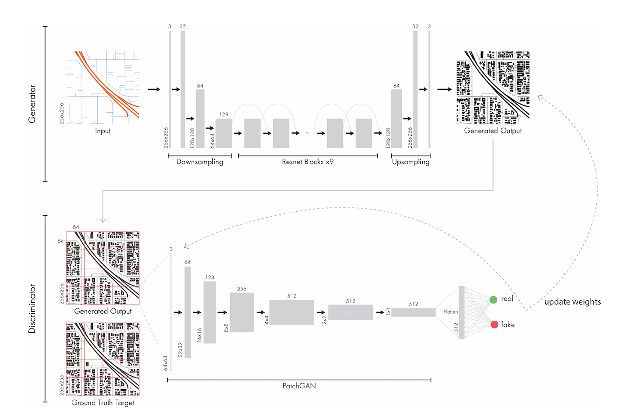 Figure 1: Used architecture during the experiments3
Additional Parameters:
Some further and also important parameters will be noted in bullet point form:
- In our configuration the loss function BCEWithLogitsLoss() from PyTorch is implemented7. This loss function combines a Sigmoid layer and the Binary Cross Entropy between the target and the input probabilities. The according formula can be found in the documentation of PyTorch7. This loss function was also used in the original GAN paper8.
- To adjust the weights and maximize the loss function the Adam optimizer with a starting learning rate of 0.0002 was chosen9.
- The training time for each experiment was 300 epochs in total with a learning rate decay after 150 epochs.
Results
With these default parameters and the number and type of pre-processed data, some intermediate results could be generated during the training process and using the test data. First, the results during the training are shown. This is followed by the results after training based on the test data set. Here, only the results of the data set with high population density are shown, since no reasonable results could be produced for the other data sets. Finally, we briefly look at the development of the loss function for the generator and discriminator.
Training Samples
In the Figure below, from left to right, the evolution of selected fake images during the training process is shown. Vertically, examples of the individual different data sets are shown. It can be seen that in the course of the process, further and sharper building floor plans could be generated. Thereby, the three data sets differ from each other as to when the respective sharpness occurs. The comparison with the real data also shows that the generation of the images becomes more realistic over the epochs (not shown here).
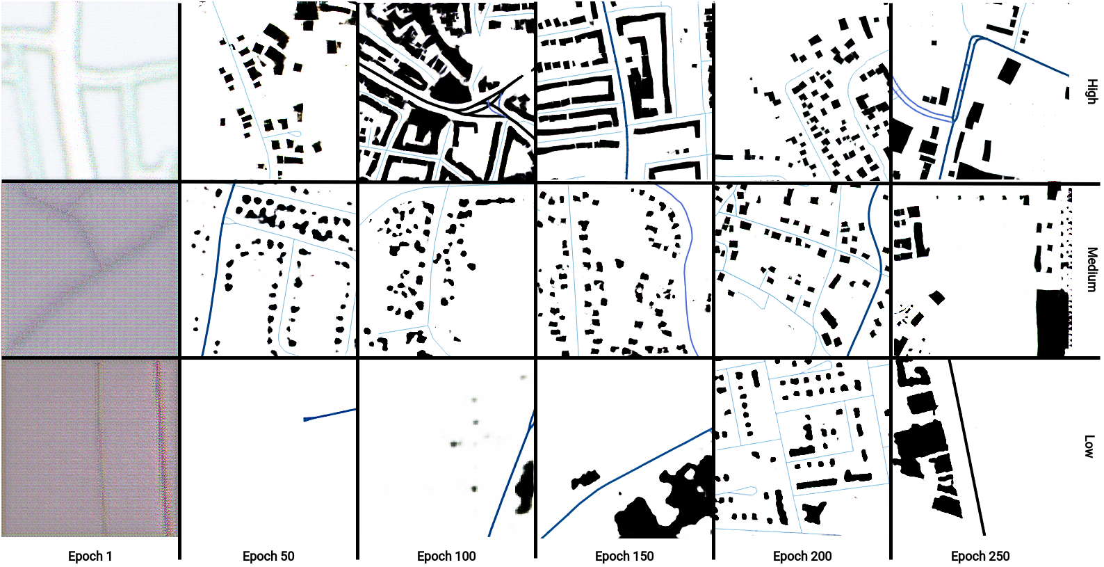 Figure 2: Sample of output during the training process for three different models
Test Samples
Since the results of the training data are already known to the model, the model was evaluated with the test data. All three models generated were tested for all data sets. However, the results of the medium and low population density datasets were without usable results. Accordingly, only the test data from the high population density dataset is used here. Only visual results without metrics were generated.
As can be seen from the figure below, it can first be determined that building footprints could be generated. When comparing the generated fake images and the real images, it becomes clear that they differ from each other. The fake images often have smaller footprints compared to the real images. The morphology is also often different. The model depicts the buildings more along the streets. In reality, especially larger buildings are between two streets.
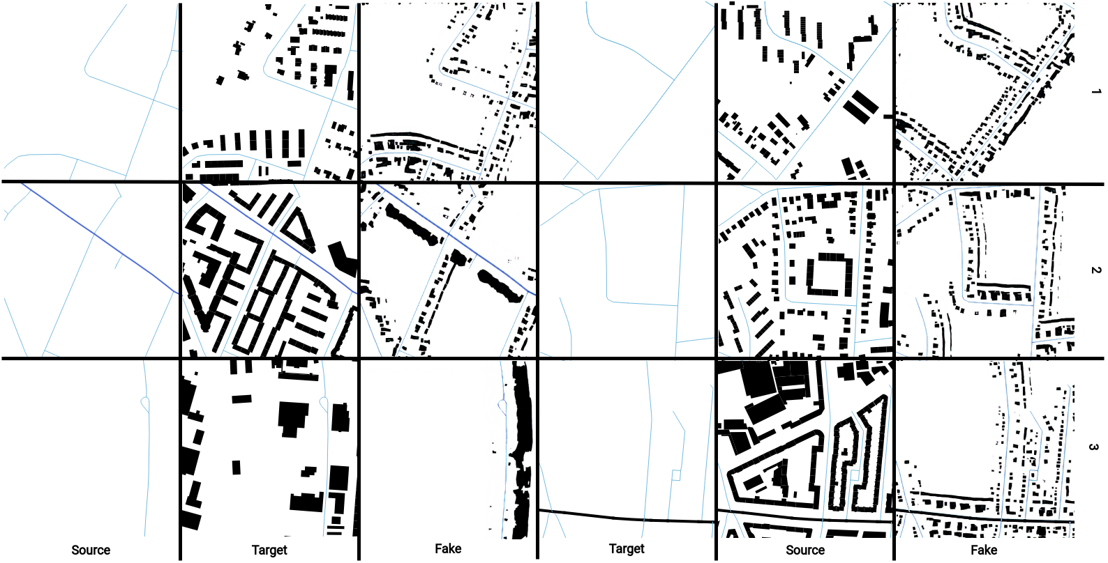 Figure 3: Sample test data results for high model
Loss Curve
Next to the pure visual output of the model, the way of the training process can be inspected with the loss curve. The evolution of the loss function can be seen in Figure 4. The development of the loss function of the generator goes down at first and increases continuously from about epoch 20. The maximum value is about nine. For the discriminator, the loss function decreases continuously for both the true and fake images.
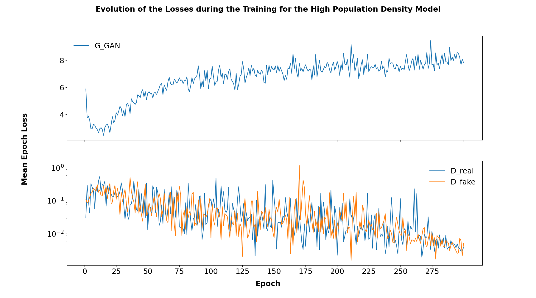 Figure 4: Evolution of the loss function for the high-density model
Interpretation
With these default parameters and the number and type of pre-processed data, it was not possible to generate satisfactory results overall, especially when it is considered that only one reasonable result could be shown here. Therefore, our objectives could not or just partly be answered. The existing result is far from perfect, but it shows the possibilities that such a model can have. To achieve more accurate results, the parameters and input data would probably have to be varied. However, in our case, no further tests were possible due to the limited computing capacity.
When the existing model is evaluated, it quickly becomes apparent that the loss function does not correspond to that of a stable converging GAN. An example of a stable GAN can be taken from Figure 5. For our application only the upper graph is relevant or corresponds to our loss curve. If now looking at what form of convergence failure is present here, reference can be made to the same blog entry/tutorial10. The copied Figure 6 shows is comparable to the loss function here. Thus, it can be taken away that in principle a model should be possible, but in this case, the optimization medium Adam is likely to be too aggressive.
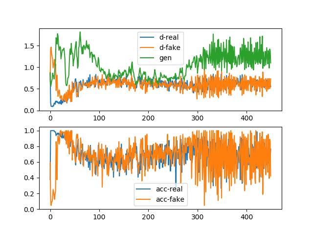 Figure 5: Line plots of loss and accuracy for a stable generative adversarial network10
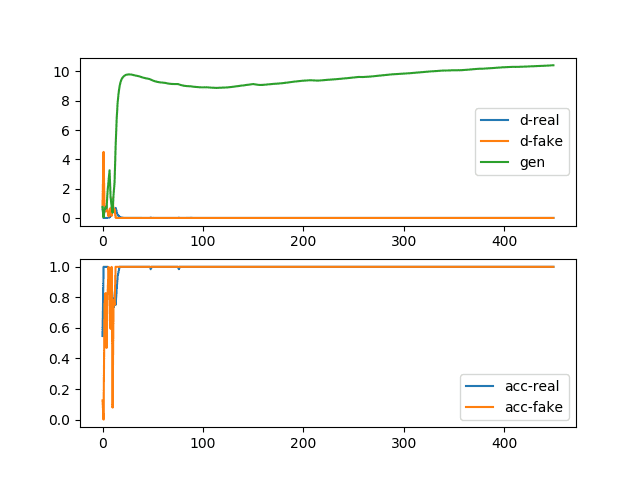 Figure 6: Line plots of loss and accuracy for a generative adversarial network with a convergence failure due to aggressive optimization10
| Flag name | Self description | Default value | Used value |
|---|---|---|---|
| model | - | pix2pix | pix2pix |
| ngf | # of gen filters in the last conv layer | 64 | 64 |
| ndf | # of discrim filters in the first conv layer | 64 | 64 |
| netD | specify discriminator architecture [basic | n_layers | pixel]. The basic model is a 70x70 PatchGAN. n_layers allows you to specify the layers in the discriminator | basic | basic |
| netG | specify generator architecture [resnet_9blocks | resnet_6blocks | unet_256 | unet_128] | unet_256 | resnet_9blocks |
| norm | instance normalization or batch normalization [instance | batch | none] | instance | batch |
| init_type | network initialization [normal | xavier | kaiming | orthogonal] | normal | normal |
| init_gain | scaling factor for normal, xavier and orthogonal. | 0.02 | 0.02 |
| no_dropout | no dropout for the generator | store_true | False |
| serial_batches | if true, takes images in order to make batches, otherwise takes them randomly | store_true | False |
| batch_size | input batch size | 1 | 1 |
| load_size | scale images to this size | 512 | 260 |
| crop_size | then crop to this size/td> | 512 | 256 |
| n_epochs | number of epochs with the initial learning rate | 150 | 150 |
| n_epochs_decay | number of epochs to linearly decay learning rate to zero | 150 | 150 |
| beta1 | momentum term of adam | 0.5 | 0.5 |
| lr | initial learning rate for adam | 0.0002 | 0.0002 |
| gan_mode | the type of GAN objective. [vanilla| lsgan | wgangp]. vanilla GAN loss is the cross-entropy objective used in the original GAN paper. | lsgan | vanilla |
| pool_size | the size of image buffer that stores previously generated images | 50 | 0 |
| lr_policy | learning rate policy. [linear | step | plateau | cosine] | linear | linear |
| lr_decay_iters | multiply by a gamma every lr_decay_iters iterations | 50 | - |
Table 1: Main parameters for the training of the GANmapper repository including their default value and our tested value
References
-
Federal Ministry of Transport and Digital Infrastructure (BMVI)(2021): Regional Statistical Spatial Typology for Mobility and Transport Research (RegioStaR). https://bmdv.bund.de/SharedDocs/DE/Anlage/G/regiostar-raumtypologie-englisch.pdf?__blob=publicationFile ↩
-
Bergstra, J & Y. Bengio (2012): Random search for hyper-parameter optimization. J. Mach. Learn. Res. 13, pages 281–305, page 281-282. ↩
-
Wu, A. N. & F. Biljecki (2022): GANmapper: geographical data translation. International Journal of Geographical Information Science. 36(7), pages 1394-1422 ↩ ↩2 ↩3
-
Isola, P., Zhu, J.-Y., Zhou, T. & A. A. Efros (2017): Image-to-Image Translation with Conditional Adversarial Networks. IEEE Conference on Computer Vision and Pattern Recognition (CVPR), Honolulu, pages 5967-5976. ↩ ↩2 ↩3
-
Goodfellow, I., Begio, Y. & A. Courville (2016): Deep Learning. MIT Press, page 499. ↩
-
He, K.,Zhang, X.,Ren, S. & J. Sun (2016): Deep Residual Learning for Image Recognition, IEEE Conference on Computer Vision and Pattern Recognition (CVPR), Las Vegas, NV, USA, 2016, pages 770-778, page 3. ↩ ↩2
-
PyTorch (2023): BCEWITHLOGITSLOSS - PyTorch Documentation. https://pytorch.org/docs/stable/generated/torch.nn.BCEWithLogitsLoss.html ↩ ↩2
-
Goodfellow, I. J., Pouget-Abadie, J., Mirza, M., Xu, B., Warde-Farley, D., Ozair, S., Courville, A. & Y. Bengio(2014): Generative Adversarial Networks. https://arxiv.org/abs/1406.2661 ↩
-
Kingma D.P. & J.Ba (2017): Adam: A Method for Stochastic Optimization. https://arxiv.org/abs/1412.6980 ↩
-
Brownlee, J. (2019): How to Identify and Diagnose GAN Failure Modes. https://machinelearningmastery.com/practical-guide-to-gan-failure-modes/ ↩ ↩2 ↩3