To answer the research question, two different approaches for data preparation and later training of the model were performed (cf. Methods). Both approaches aim to include the known requirements and known information from the original GANmapper article1. The second attempt could not be tested afterwards, but it is a further development of the first approach and accordingly takes over large parts of the first approach. The background of why the second approach could not be tested in practice is explained in the Discussion section.
Known Requirements from the GANmapper Paper
As it is already known, within the Ganmapper paper different experiments were tested with respect to the data and their configuration. Here we only follow their best results in order to avoid duplicate experiments. From the paper, the most promising settings can be summarized as follows:
- OpenStreetMap (OSM) building footprints and street data are used as a data basis
- Converting basic street data to Coloured Road Hierarchy Diagrams (CRHD) proposed by Chen et al. (2021)2
- Using not all street types from OSM
- Zoom level 16 of the Slippy map format/XYZ-Tiles as a compromise between visual sharpness and contextual information
- Source and target data pairs
- 256x256 resolution per source and target tile
First Approach
First, the OSM data of Hamburg, Lower Saxony, and Schleswig-Holstein were downloaded from the website of www.geofabrik.de and merged to one layer3. Subsequently, the streets and building footprints were trimmed to the minimum bounding box of the administrative boundaries of Hamburg. In order to differentiate by population densities, corresponding data was downloaded from eurostat4 and cropped. The subdivision by population densities was done by dividing the Eurostat data set into three quantiles (<33%,>33%-<66%,>66%). This is a first approximation to simplify a subdivision into low, medium, and high population density areas. The corresponding distribution including the threshold values can be seen here:
 Figure 1: Histogram of the population density of Hamburg and surroundings including three quantiles in 2018
The subdivision leads into this following map:
Figure 1: Histogram of the population density of Hamburg and surroundings including three quantiles in 2018
The subdivision leads into this following map:
 Figure 2: Area of interest and the according population density (light green line shows administrative boundaries of Hamburg)
Subsequently, the street and building data were cut by the respective population density. Before the XYZ tiles could be generated as source and target data pairs, the streets and buildings had to be visualized according to the specifications. With respect to the buildings, the footprints were simply colored black. For the different street types that are represented as CRHD, the GitHub Repository by Chen et al. (2021)2 was used. For this, the assumption had to be made that the authors of the GANmapper paper used exactly the corresponding street lines and colors. In terms of line width, the ratios of the repository were picked up and the starting width was estimated. Subsequently, the source and target data for each population density could be generated. Some examples can be seen here:
Figure 2: Area of interest and the according population density (light green line shows administrative boundaries of Hamburg)
Subsequently, the street and building data were cut by the respective population density. Before the XYZ tiles could be generated as source and target data pairs, the streets and buildings had to be visualized according to the specifications. With respect to the buildings, the footprints were simply colored black. For the different street types that are represented as CRHD, the GitHub Repository by Chen et al. (2021)2 was used. For this, the assumption had to be made that the authors of the GANmapper paper used exactly the corresponding street lines and colors. In terms of line width, the ratios of the repository were picked up and the starting width was estimated. Subsequently, the source and target data for each population density could be generated. Some examples can be seen here:
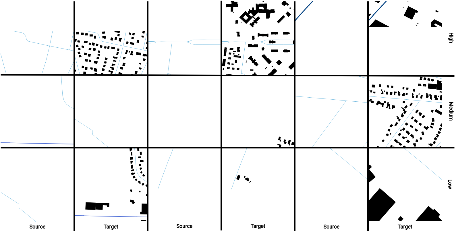 Figure 3: Example training data for the first approach
These data pairs were pre-processed in the last step using the existing script. The main steps of the process were:
Figure 3: Example training data for the first approach
These data pairs were pre-processed in the last step using the existing script. The main steps of the process were:
- Sorting out images without building footprints.
- Sorting out images with few building footprints or in general images with more white pixels included. The described values of the repo of a maximum of 170000 white pixels at zoom level 16 were used, i.e. with
- In the next step, the total data was divided into training, testing and validation data (70%,15%,15%).
- At last, the source and target data were merged to form a larger image.
After pre-processing starting from a total amount of about 12600 source images, the number of image pairs per population density can be obtained from Table 1.
| Population Density | Tiles after removing blank tiles | Training tiles after pre-processing |
|---|---|---|
| High | 3765 | 1758 |
| Medium | 3110 | 311 |
| Low | 1690 | 72 |
Table 1: Number of data pairs after pre-processing per population density
Drawbacks of the First Approach
Although this approach was used, and the results were partly generated by means of these data, it was already determined in the course of the processing that there are some disadvantages, which are to be explained here already, in order to show afterward the alternative and improved approach to the generation of data. First of all, the up-to-dateness and especially the spatial resolution of the population data must be criticized. The spatial resolution leads to border effects where areas of the individual population polygons of the raster tiles are cut off (cf. Figure 3). In addition, within the population distribution, partly no data are available (cf. Figure 2), whereby this does not include of course that there can be no buildings. Thus, such cropping of the data already leads to the loss of possible training data. In addition, it can be seen from Table 1 that the sorting out of images with insufficiently colored pixels leads to a very small number of training pairs and that the existing training pairs within the population density classes look mostly similar regarding the morphology. Thereby, the amount of training data are probably not sufficient for an ordinary training process. The impact on comparability between datasets and the general impact on the question will be addressed in more detail in discussion. The last thing to criticize is the use of only the proposed street types. Only eleven of 28 possible street types in Hamburg were used.
Changes for the Second Approach
Regarding the number of disadvantages and the missing comparability due to the different amounts of training data, it seems to be reasonable to change the pre-processing. The basic process remains the same, but the division was not based on the population density of a dataset, but solely on the pixel distribution. Secondly, the street types were examined more closely and additional street types were added.
Before the distribution of the white pixels could be examined in more detail, it was first necessary to determine which street types of the OSM data should be used. The summation of the lengths results in the following figure:
 Figure 4: Histogram of the length of different street types in Hamburg and surroundings
In the previous approach were already used, the following street types:
Figure 4: Histogram of the length of different street types in Hamburg and surroundings
In the previous approach were already used, the following street types:
street_types = ['service', 'residential', 'tertiary_link', 'tertiary', 'secondary_link', 'primary_link',
                 'motorway_link', 'secondary', 'trunk', 'primary', 'motorway']
Based on the distribution it was decided to add ‘unclassified’ and ‘living_street’. Many of the street segments with shorter path lengths, such as ‘bridleway’ were not used due to these. For other street classes, such as ‘cycleway’ or ‘footway’ the visual check seemed to show a lot of duplication with the other street types. In addition, these street types seemed, based on our local knowledge, to be not complete in large parts. Subsequently, XYZ tiles were generated again with slightly increased line thickness.
Subsequently, the data set had to be divided. The following figure shows the accumulation of white pixels within the entire initial data set including the division into three quantiles.
![]() Figure 5: Histogram of the total amount of white pixels in Hamburg and surroundings
Figure 5: Histogram of the total amount of white pixels in Hamburg and surroundings
Thereby the number of pixels without color value becomes clear by for example waters or forests. Subsequently, these values were used to perform a slightly modified pre-processing with the corresponding quantile values. Accordingly, the adapted function can be seen in Listing 1. Basically, we have just changed the condition to sort the data in different folders with different pixel values. This is the only changed code part in the whole project.
def combine_target_mask(mask_file_path, target_file_path, threshold_1,threshold_2, output_folder_high, output_folder_medium, output_folder_low,i):
    img1 = cv2.imread(mask_file_path)
    img2 = cv2.imread(target_file_path)
    # resize
    img1 = cv2.resize(img1, (256,256))
    img2 = cv2.resize(img2, (256,256))
    # high
    if np.unique(img2, return_counts=True)[1][-1] > threshold_1:
        h1, w1 = img1.shape[:2]
        h2, w2 = img2.shape[:2]
        #create an empty matrix
        vis = np.zeros((max(h1, h2), w1+w2,3), np.uint8)
        #combine 2 images
        vis[:h1, :w1,:3] = img1
        vis[:h2, w1:w1+w2,:3] = img2
        cv2.imwrite(output_folder_high + str(i) + '.png', vis)
    # medium
    elif np.unique(img2, return_counts=True)[1][-1] <= threshold_1 and np.unique(img2, return_counts=True)[1][-1] >= threshold_2:
        h1, w1 = img1.shape[:2]
        h2, w2 = img2.shape[:2]
        vis = np.zeros((max(h1, h2), w1+w2,3), np.uint8)
        vis[:h1, :w1,:3] = img1
        vis[:h2, w1:w1+w2,:3] = img2
        cv2.imwrite(output_folder_medium + str(i) + '.png', vis)
    # low
    elif np.unique(img2, return_counts=True)[1][-1] < threshold_2:
         h1, w1 = img1.shape[:2]
         h2, w2 = img2.shape[:2]
         vis = np.zeros((max(h1, h2), w1+w2,3), np.uint8)
         vis[:h1, :w1,:3] = img1
         vis[:h2, w1:w1+w2,:3] = img2
         cv2.imwrite(output_folder_low + str(i) + '.png', vis)
    else:
         vis = None
    return vis
Listing 1: Changed combine_target_mask function for the second approach With this type of pre-processing, the population density is only indirectly inferred and the pixel density, especially since streets are also included, is only an indicator for a high population density. However, the following figure shows that at least in parts a lower population density should apply. In addition, compared to the first approach, the artifacts could be almost completely eliminated by splitting. A comparable effect can also be found in the number of training data in Table 2.
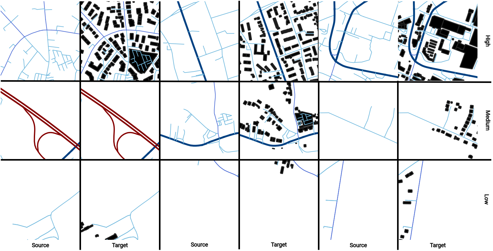 Figure 6: Example training data for the second approach
| Amount of Colored Pixels | Train Dataset | Test Dataset | Validation Dataset |
|---|---|---|---|
| High | 2503 | 313 | 313 |
| Medium | 2503 | 313 | 313 |
| Low | 2578 | 322 | 323 |
Table 2: Number of data pairs after pre-processing by pixel value
References
-
Wu, A. N. & F. Biljecki (2022): GANmapper: geographical data translation. International Journal of Geographical Information Science. 36(7), pages 1394-1422 ↩
-
Chen, W., Wu, A., N. & F. Biljecki (2021): Classification of urban morphology with deep learning: Application on urban vitality. Computers, Environment and Urban Systems. 90(101706). ↩ ↩2
-
Effective date of OSM: 2023-06-06 ↩
-
Batista e Silva F, Dijkstra L, Poelman H (2021): The JRC-GEOSTAT 2018 population grid. JRC Technical Report. Forthcoming. ↩